Navigation

State Machine

State Machine Diagram

Note: State machine diagrams can be generated using the state machine visualizer tool. When using the tool, we sometimes have two separate transitions that are representing the same state change, meaning you may see “duplicate” arrows.

run: ros2 run mrover visualizer.py in order to have live visualization of what’s going on in the state machine.

What is a State Machine?

A state is an object that defines a certain mode of behavior for a system. We can define a state through its behavior and also its transitions. For our purposes, the Navigation system can be “in” exactly one state at any given time. Every time one cycle of the system occurs, we execute the logic of the current state, and then at the end of that execution, we transition into a new state. This new state does not need to be a different state (in fact, most of the time the “new” state is just the same state). In this system, we can create complex behavior in an organized and relatively easy-to-think-about manner. Many times, state machines are created “manually” through code that looks something like this:

switch (state) {
    case StateOne:
       action()
       if action_complete:
           state = StateTwo
       else if action_failed:
           state = StateThree
       else:
           state = StateOne
       break
    case StateTwo:
       print("complete")
       state = StateTwo
       break
    case StateThree:
      print("failed :(")
      state = StateThree
      break
}

This is probably fine in simple cases such as the one above but when state machines get big and complicated the logic can very quickly get hairy and hard to debug. The solution to this is to rethink what a state really is on a more fundamental level: an object. Every state in a given state machine shares many properties. Every state has some action that gets run and every state can transition into other states. If we implemented each state as an object that inherits from some base class with a function that runs the action and returns some transition, we can then map those transitions to output states and implement that actual logic for putting together the state machine itself just once. In other words, we create the abstraction of states just once for any general state machine, and then we can put together an arbitrarily large state machine just by thinking of it one state at a time.

We use a custom state machine implementation giving us control over the specific requirements of the system. Each state inherits from a base State class and implements three core methods:

• on_enter(context): Called when entering the state
• on_exit(context): Called when exiting the state
• on_loop(context): Called each iteration while in the state, returns the next state

This custom implementation provides clean separation of concerns, easy debugging, and maintainable code while being tailored specifically for our navigation requirements.

State descriptions

Off State

Off State is the default state of the state machine and it indicates that the navigation system is currently off. It does nothing. Importantly, it does NOT send out zero velocity commands as those would overlap with valid velocity commands from teleop. We switch out of the Off State and into the Waypoint State if we receive a request to enable auton which can be inferred from the course object being not None.

Done State

Done state may seem similar to the off state but it is not the same. We switch into the Done State when we have completed the objective provided by teleop GUI or after we have given up on that objective. We send out zero velocity commands in this state because the rover is still enabled and we don’t want it to move even under teleop controls until it is disabled. However we will switch back into waypoint state if we receive a new course in this time. The meaning of this is that we technically do not have to turn auton off (from the gui) in order to start a new objective.

Waypoint State:

Summary: The Waypoint State was created to command the rover along a course of waypoints.

Actions (Published messages): The Waypoint state publishes drive commands (Twist messages) that are calculated via the get_drive_command function. It will use the waypoint_indexth waypoint in the course as input to the get_drive_command function and if the get_drive_command function returns true, we have reached the current waypoint so we then increment the waypoint_index variable.

The state also supports A* path planning with costmap integration when enabled. It maintains separate trajectories for waypoint navigation and A* path planning, and updates path planning periodically based on the UPDATE_DELAY parameter.

Transitions:

• If the waypoint at waypoint_index is None: transition into the done state
• If we are at a target from a previous leg: Transition into the Backup state (to avoid driving through the previous leg’s target)
• If we see the target (via a message from perception): Transition into the Approach Target state
• If we see the target in the long range camera: Transition into the Long Range state
• If we complete a waypoint with a target associated with it: Transition into Costmap Search state
• If the rover is stuck: Transition into Stuck Recovery state
• Else: Stay in Waypoint State

Approach Target State:

Summary: The Approach Target State was created to command the rover towards a target.

Actions (Published messages): The Approach Target state publishes drive commands (Twist messages) that are calculated via the get_drive_command function. It uses the position of the spotted AR tag as the position input to the get_drive_command function and if the function returns true, we have reached the AR tag so we exit the state.

The state also supports A* path planning with obstacle avoidance when costmap integration is enabled. It updates target position and path planning periodically to handle moving targets.

Transitions:

• If the target position is None for a long period of time: Return to the previous state (Search/Waypoint state)
• If we have arrived at the target: Return Done state
• If the rover is stuck: Transition into Stuck Recovery state
• Else stay in Approach Target State

Long Range State:

Summary: The Long Range State commands the rover towards targets detected by the long-range camera using bearing information.

Actions (Published messages): Similar to Approach Target State but specialized for long-range camera data. It processes ImageTargets messages from the long-range camera and uses bearing information to project target positions ahead of the rover. It avoids high-cost areas when projecting target positions.

Transitions:

• If the target is detected by the ZED camera (higher precision): Transition into Approach Target State
• If the target is lost and search is needed: Transition into Costmap Search State
• If the rover is stuck: Transition into Stuck Recovery state
• Else stay in Long Range State

Search State

Summary: The search state is used when the rover arrives at a given waypoint where an object is expected to be located, but wasn’t able to detect the object on the way there. To do this, the rover will follow a search spiral. If the cost map is utilized, the search spiral is modified where the rover will take a lower cost (a route that avoids obstacles). This lower cost route is found with a custom implementation of the A* algorithm. The algorithm uses an occupancy grid that shows the cost of each cell. After the algorithm adds the cost of distance from the search spiral and other factors that contribute to the rover getting stuck.

Actions: The Search state publishes drive commands (Twist messages) that are calculated via the get_drive_command function. It uses the position of the next point in the search pattern as the position input and the costmap to develop a custom path to follow, and calls the get_drive_command function. If the function returns true we have reached the next point in the search pattern so we increment our path index. Once the path index is equal to the length of the path, we have traversed the entire search pattern and just give up.

Transitions:

• If a target is detected during search: Transition into Approach Target State
• If a target is detected by long-range camera: Transition into Long Range State
• If the search pattern is complete without finding target: Transition into Done State
• If the rover is stuck: Transition into Stuck Recovery state
• Else stay in Costmap Search State

Backup State

Summary: The Backup state is entered into after we complete a search for a target (e.g. the tag). We enter this state because after arriving at a target, as we move onto another leg, we don’t want to run over the previous target. Instead we opt to retrace the rover’s path backwards for some distance to lower the odds of collision with a target.

Actions: The Backup state publishes drive commands (Twist messages) that are calculated via the get_drive_command function using the position of all previous points in the rover’s path history. It creates a reverse trajectory from the rover’s recorded path history and drives backwards along the recorded path for a specified distance.

Transitions:

• Returns to the Done state if there are no more waypoints to traverse to in the course
• Else returns to the Waypoint State

Stuck Recovery State

Summary: The Stuck Recovery state implements sophisticated recovery behaviors when the rover is detected as stuck.

Actions: The state implements a J-turn recovery maneuver consisting of two phases:

1. Phase 1: Drives backwards to a point behind the rover
2. Phase 2: Performs a J-turn by driving backwards to a point at a 45-degree angle

The state includes timeout protection to prevent infinite recovery attempts and resets stuck detection when recovery is complete.

Transitions:

• If recovery is complete or timeout is reached: Return to the previous state
• Else stay in Stuck Recovery State

Context

Context is a class that holds many common functions and variables between the states. It serves as the bridge between the Navigation node and the other ROS nodes. The context class also holds references to an object of the Rover class as well as an object of the Environment class and Course class. The Rover class deals with all data related to the rover, the environment class deals with all data related to the environment surrounding the rover. See below for a list of important functions in the Context, Rover, Environment, and Course

Context Functions/Attributes

• course: Course object (see Course description)
• env: Environment object (see Environment description)
• rover: Rover object (see Rover description)
• drive: DriveController object (see DriveController description)
• disable_requested: boolean indicating that a disable has been requested and has not yet been processed

Course

The course class keeps track of the rover’s course. A course is essentially just a managed queue of waypoints that represent where the rover needs to drive. Each waypoint also maintains information regarding what target it is associated with as well as what the rover should do after reaching said waypoint

Functions/Attributes

• increment_waypoint() increments the saved waypoint index in the course that the rover is currently trying to follow
• waypoint_pose(wp_idx) -> SE3 returns an SE3 pose object representing the pose of the waypoint at the specified index in the active course
• current_waypoint() -> Optional[Waypoint] returns the object (or none) of the current waypoint
• is_complete() -> Bool returns True if the rovers waypoint index is past the number of waypoints in the course

Environment

The environment class keeps track of data regarding the environment around the rover.

Functions/Attributes

• get_target_pos(frame) -> Optional[np.ndarray] returns the position (as a numpy array) of the target specified in the frame param from the tf tree, or none if there is no tag with that id in the tf tree
• current_target_pos() -> Optional[np.ndarray] returns the position of the target frame associated with the current waypoint (or none) if we don’t have one

Rover

The rover class keeps track of the interface regarding the rover itself

Functions/Attributes

• get_pose()->SE3 returns the pose of the rover as an SE3
• send_drive_command(Twist) sends a twist command to the rover
• send_drive_stop() tells the rover to stop

Trajectory

The Trajectory class is an abstract class that we use to represent a planned path that the rover takes. It is made up of a list of coordinates (still an np array) and maintains an internal pointer to the current point that the rover is on in the list. The base functions of getting the current point (get_current_point) and incrementing the point (increment_point) are implemented in the base class itself. Below is the documentation regarding the SearchTrajectory class.

SearchTrajectory

The SearchTrajectory is a trajectory that is created to represent a search pattern for the rover. It will generate a list of coordinates representing target positions along a 2D square spiral emanating outwards from the waypoint using the following function. (this is copy-pasted directly from the code)

# The number of spirals should ensure coverage of the entire radius.
num_spirals = np.ceil(coverage_radius / distance_between_spirals).astype("int") + 1
# The angles are evenly spaced between 0 and 2pi*num_segments_per_rotation
angles = np.linspace(0, 2 * np.pi * num_spirals, num_segments_per_rotation * num_spirals + 1)

# Radii are computed via following polar formula.
radii = angles * (distance_between_spirals / (2 * np.pi))

# Convert polar to Cartesian coordinates
x_coords = np.cos(angles) * radii
y_coords = np.sin(angles) * radii
vertices = np.hstack((x_coords.reshape(-1, 1), y_coords.reshape(-1, 1)))

Path Planning

A* Algorithm

The navigation system uses a custom A* implementation for path planning with comprehensive costmap integration. At each step, A* evaluates a current node by combining two values: g(n) and h(n).

• g(n) - the actual cost to reach the current node n from the starting point
• h(n) - a heuristic estimate of the cost from the current node n to the ending point

Each node is then given a value based on the following algorithm: f(n) = g(n) + h(n). When making a path A* considers 8 different directions which can be represented by the 8 directions on a compass.

Features:

• Costmap Integration: Uses occupancy grid data for intelligent obstacle avoidance
• Heuristic Functions: Multiple heuristic options optimized for different scenarios
• Path Smoothing: Post-processing algorithms for smoother trajectories
• Failure Handling: Graceful handling of path planning failures with fallback strategies

Key Classes:

• AStar: Main path planning algorithm implementation
• SpiralEnd: Exception for spiral completion scenarios
• NoPath: Exception for path planning failure cases
• OutOfBounds: Exception for out-of-bounds coordinate requests

Algorithm Characteristics:

• Optimal Path Finding: Guarantees optimal paths when possible
• Obstacle Avoidance: Intelligently routes around detected obstacles
• Cost Optimization: Minimizes traversal cost while maintaining safety
• Real-time Performance: Optimized for real-time navigation requirements

Path Smoothing

Since A* generates a sequence of grid like points (only considers 8 directions at each node), the sequence it outputs is generally jagged and dense. To improve upon this path, we use post-processing algorithms to give a smoother trajectory. Path smoothing can be found in smoothing.py and the function smoothing() is used to smooth a given trajectory generated by A*. Within this function there are two post-processing algorithms used. Both are toggleable based on our .yaml files, as well as operator input from the GUI.

Path Relaxation

The first post-processing algorithm is path relaxation. Our implementation uses a greedy point-removal algorithm that repeatedly removes points whose removal has the lowest cost. This helps eliminate unnecessary points that would otherwise increase the rover’s driving time.

Path Interpolation

The second post-processing algorithm is path interpolation. During path interpolation, we fit a curve to the given trajectory and then resample points along that curve. Because A* generates a jagged path, interpolation produces a more finely tuned trajectory.

DriveController Class

The DriveController class is responsible for converting a target position or path into a Twist command. It contains two different driving approaches: the Drive Controller State Machine and Adaptive Pure Pursuit. When Pure Pursuit is not used, the Drive Controller uses its internal state machine to determine the rover’s driving behavior.

get_drive_command function

The get_drive_command function is used by many states and its job is to determine the Twist command to send the rover to a desired point. It automatically traverses to intermediate targets if the straight-line path to the ultimate target crosses through one or more FailureZones (see FailureZone and PathPlanner documentation below).

Its signature is as follows: def get_drive_command( self: DriveController, target_pos: np.ndarray | Trajectory, rover_pose: SE3, completion_thresh: float, turn_in_place_thresh: float, drive_back: bool = False, path_start: np.ndarray | None = None, last_point: bool = True, ) -> Tuple[Twist, bool]:

Inputs:

• The target position (a 3D position vector) or a Trajectory
• The Rovers pose as an SE3 object
• A completion threshold (in meters)
• A turn-in place threshold (representing the minimum angle between the rover’s direction and the vector towards the target position allowed before we begin driving straight and outside of which we turn in place)
• drive_back represents whether we are driving backwards or not
• path_start represents the start of a line segment for path following (optional)
• last_point if a trajectory is given for the target_pos, this parameter is given if the rover is at its last point

Output:

• A Twist message containing the desired command velocities for the left and right sides of the drivetrain
• A boolean that is true if the drive is complete and false if it is not complete

Drive Controller State Machine

When the cost map is not being used, we are at the last point in a trajectory, or an operator chooses to disable pure pursuit, the get_drive_command uses our state machine to drive the rover. When using this, the rover has three different states: DriveMode.STOPPED, DriveMode.TURN_IN_PLACE, or DriveMode.DRIVE_FORWARD. The rover never turns and drives forward simultaneously. Although this implementation is relatively simple, it ensures that the rover reaches a given point without oscillating compared to other drive controller approaches.

Driver State:

• last_angular_error (Optional[float]) represents the angular error that was recorded at the most recent call to the get_drive_command function. It is initialized as None
• driver_state (DriveMode) is an enum that is either DriveMode.STOPPED, DriveMode.TURN_IN_PLACE, or DriveMode.DRIVE_FORWARD. It is initialized as None.

Reason for the Drive Controller State Machine

Summary of previous drive algorithm: The previous drive algorithm was quite simple. At a high level, we start by turning to face the (potentially intermediate) target point and then drive straight towards it. This is implemented via calculating first whether we are within the tolerance of facing towards the target (and if we are we add an x component to the output vector) and then calculating a corrective turning factor based on our angular offset from our current direction vector and the vector facing towards the target. This will result in us either driving towards the target while trying to correct for any angular errors if we are within the dot-product tolerance or just simply turning in place until we are within the dot-product tolerance.

However this basic algorithm is not quite enough to get the desired behavior in all cases. In testing we found that the rover tends to oscillate in some situations (namely - when we are driving in the odom frame) this is likely because of latency in the odom frame measurements. This latency is undesirable but some amount is unavoidable so we require workarounds to stop oscillations. The primary one that we settled on was using the intermediate value theorem (IVT). Basically, if the sign of our error changes, we know that we have passed through zero and can essentially just ‘give up’ right there. We use this for our angular error (which is where the oscillation was) if the sign of our angular error changes: we stop trying to turn in place (even if we are still outside the turn in place threshold).

This is the reason why the function was refactored into a class and the last angular error is maintained. But then why did we build a state machine? It seems like on a surface level this is not that hard of a change to make because we can just add an extra check to our existing logic for not turning anymore. However the problem comes when evaluating the logic for going from driving straight to turning in place. If we continue to use the previous logic of turning in place whenever the angular error is outside of the threshold you end up at exactly the same problem,the sequence of events is as follows: From iteration 1 to 2 you switch angular error signs and then use IVT to recognize that we have done so and start driving straight, the next iteration of the loop (iteration 3) the error is of the same sign as it was in the last one but still outside of turn_in_place_thresh thus we switch to turning in place and once again begin oscillating albeit this time with a iteration in between each swing. To prevent this, we can instead switch to turning_in_place only on the rising edge of the turning error. What this means is we only switch from driving straight to turning in place if the previous error was inside of the tolerance and the current error is outside of the tolerance, this prevents us from oscillating in the aforementioned case because in both cycle 2 and 3 we would have been outside of the tolerance and thus not hit the rising edge.

All of this logic can be a bit dizzying, so we decided that it would be cleanest and easiest to understand if the drive code was refactored into a state machine. Below is a diagram of the state machine.

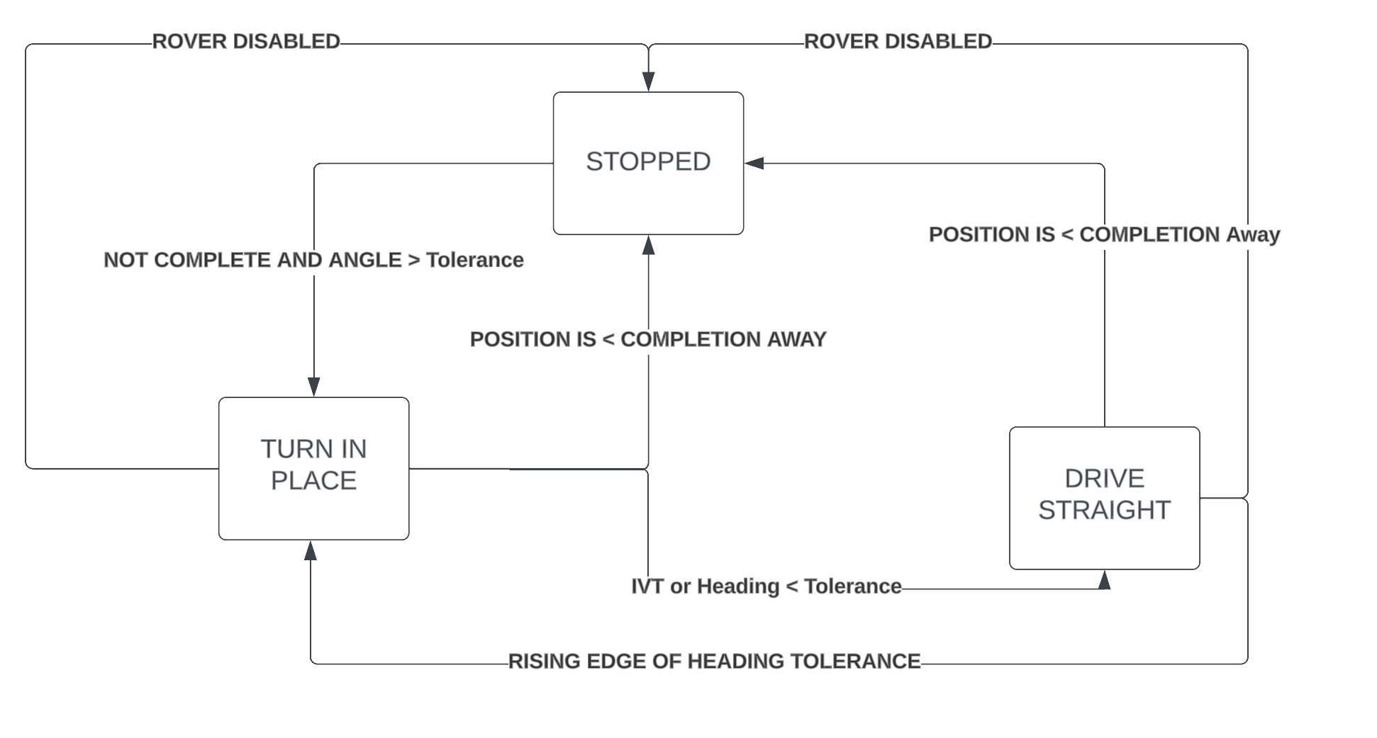
The logic in the code is written to follow the state machine diagram. At a high level the rover flows from being stopped until it has a target farther away then completion_distance to turning in place until it is either within angular tolerance or IVT, and then driving towards it until it arrives, with early escapes for arriving and disabling. The actual control logic remains as described above.

Adaptive Pure Pursuit

When we are not using the Drive Controller State Machine we are instead using a version of Pure Pursuit called Adaptive Pure Pursuit. Pure Pursuit is a geometric path tracking built around the idea of “chasing” a lookahead point on the path ahead of it and then computing a curvature and corresponding angular velocity for the rover to drive along a circular arc that will intercept that lookahead point. When describing Pure Pursuit, a circle around the rover is often used to represent the lookahead distance and its intersections with the path.

When we find the intersection between this circle and the rover’s path, we choose the farthest point intersected and have the rover drive towards this point. The exact Twist that is generated differs from our Drive Controller State machine. What makes this Pure Pursuit considered adaptive is that the lookahead distance of the rover is not constant. The actual lookahead differs based on the rovers heading towards its target point. The general idea of how the drive controller works is outlined below:

If the heading of the rover directed towards the target point:

• linear velocity is at its maximum
• angular velocity is at a minimum
• lookahead distance is at a maximum

If the rovers heading is drastically away from the target point:

• linear velocity is at its minimum
• angular velocity is at a maximum
• lookahead distance is at a minimum

The exact algorithm we used was based off of a document by Purdue. Read more about that here.

Arm Controller

The ArmController is a ROS2 node that handles the robotic arm’s motion control. It takes high-level commands (like “move the end effector to this position”) and converts them into low-level joint commands that the actual arm motors can execute. The Arm Controller has three main modes: position control, velocity control, and a special “typing” mode.

Arm Diagram

Our robotic arm has 5 degrees of freedom (DOF), meaning it has 5 separate joints which control the arm’s movement.

The following diagrams represent our current arm and have been illustrated to describe its different parts:

• The red line represents Joint A
• The intersection between the red line and the green line is Joint B
• The intersection between the green line and yellow line is Joint C
• Joint D and E are the two blue cylinders just before the end effector

Each of these joints have separate limits and move the arm in different ways:

• Joint A moves the arm in the Y-axis
• Joint B and C work in combination to move the arm in the X and Z axis (if we ignore the movement of the end effector)
• Joint D and E work in combination to change the roll and pitch of the end effector

Arm IK

One of the main uses of the Arm Controller is Arm IK. IK is an abbreviation for inverse kinematics: a practice used in robotics to calculate the necessary joint positions required to place an end effector (robot’s “hand”) at a given position. In particular, the Arm Controller can convert end effector position/orientation commands into joint angles.

Another aspect of this is being able to convert velocity commands into joint velocities. This is useful as it enables us to move the arm in the Cartesian space rather than controlling each joint independently. Instead of controlling each joint separately, we are essentially able to move the end effector in directions such as forward, backward, left, right, up, or down. These directions seem simple in practice but this requires moving multiple joints. Try moving your arm in a straight line up and down. Notice how you have to move not only your elbow, but your shoulder as well!

Although Arm IK is important, the Arm Controller has the important responsibility to also monitor the arm:

• Safety checks to prevent the arm from hitting its limits
• Automatic velocity scaling if commands are too fast
• Timeout protection (stops if no commands received for 0.3 seconds)
• Real-time joint limit validation
• Forward kinematics is used to track the arm’s current position
• Arm’s current state to the TF tree for other nodes to use

For an in-depth review of the logic refer to this document: IK.pdf

Click IK

Note

Click IK has not been merged into main yet. Find it on avb/click-ik

Click IK is an extension of the existing Arm IK System that enables intuitive, point-and-click control of the robotic arm enabling operators to click on a point in the camera feed to move the arm’s end effector to that location. This system provides a more natural interface for teleoperation, particularly for the ES mission.

Click IK receives 3D position data from a perception node. The perception node is responsible for converting the clicked pixel coordinates from the GUI into a 3D point using the point cloud. To create this functionality, there is a service within the Arm Controller to determine if a clickable point is within the arm’s limits. If this point is within the arms limits, this service will move the arm towards the given point.